
Knowing if the trend is strong enough to support your position is important. The ADX is popular for assessing that. As a result, I made the ADX adaptive using a three different methods so you can experiment to find the method that leaves you with no question as to whether the ADX is set to the right length. The three methods are TOS Periodogram, Dr Ehlers' Band-Pass Filter method, and an AMA like volatility adapter using the efficiency ratio.
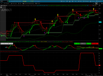
Here is a screenshot. The adaptive ADX is simply displayed here in a label on the top left corner. It also compares the "DI+" to the "DI-" to determine trend direction and color codes the label Green if ADX > 25 and "DI+" > "DI-" or Red ADX > 25 and "DI+" < "DI-". The script can easily be modified to provide a plot of the adaptive ADX values so the trend of ADX values over time can be readily seen.

Note: Articles from Dr Ehlers use arrays to normalize the periodogram data and then a center of gravity method to pin point the dominant cycle. However, thinkscript does not support arrays as needed to do the drill down further to identify the precise dominant cycle, per se. However, the cycle value provided by the periodogram in TOS appears to be capable of finding more trading opportunities than found with static fixed length values. Be sure to test it out before using it.
If you are needing cycle lengths more representative of the market dominant cycle consider using the Band-Pass Filter method which measures the market dominant cycle length by counting the bars between zero crossings of the band-pass filter waveform. The method is described in detail in Dr Ehlers book, "Cycle Analytics for Traders", chapter five. This method obtains more precise estimates of the market dominant cycle and does not bog down ThinkOrSwim with heavy duty computations. I think you will really like this one! It provided precise cycle lengths when tested against a sinewave having a fixed period length that closely matched the cycle period lengths of the sinewave. Here are a number of screenshots that capture the results:
The red line is the Dominant Cycle length measured by teh zero crossings of the band-pass filter. Zero crossings of the yellow line are watched and the number of candles between crossings are counted and multiplied by two to get the measured value of the dominant cycle length. The yellow line was made by the band-pass filter. The Cyan line is the SineWave signal of given period length = 8. As shown in the screenshot, the band-pass filter measured the period length correctly getting DC = 8.

Here are two more test cases showing the band-pass filter method gets the correct DC length for a sinewave having period = 20 and period = 40:


Because the band-pass filter method is only counting one half of the cycle then multiplying by two, it does not get the correct DC length when the sinewave has a period length that is odd. However, the values that it gets are only off by +/- 1 as shown in the test cases below.
For sinewave period = 7, the band-pass filter gets DC = 6 or DC = 8, with the correct number being the average of the two:

For sinewave period = 19, band-pass filter measures DC = 20 or DC = 18 with the correct value being the average of the two:

And finally for sinewave DC = 39, the band-pass filter measures DC = 40 or DC = 38, with the correct value being the average of the two:

Furthermore, if you are needing an ADX that adjusts to market volatility then consider using the AMA like volatility adapter method by selecting 'yes' for it and 'no' for the other two methods in the study properties dialog. The cycle length produced by this method is much shorter than the market dominant cycle value measured by the band-pass method, and I think that may be due to the current day volatility. Here is a screen shot comparing the cycle lengths produced by this volatility based method and the Band-Pass filter method, as well as the resulting ADX lines. The red ADX label in the top left corner was computed using the volatility adapter, which from the studies in the lower portion of the screen shot can be seen to have much shorter lengths leading to the higher ADX values, whereas the white ADX label was computed using the Dominant Cycle length from the Band-Pass filter method having much larger lengths, hence the lower ADX values.

In all, you now have a way to obtain dominant cycle lengths to keep in your trading arsenal that will not bog your computer down. Testing against a sinewave across a wide range of cycle lengths obtained closely matching values. This method is provided as a Script function in the code above and can readily be used to make your other indicators adaptive as desired. Happy hunting!
Here is a screenshot. The adaptive ADX is simply displayed here in a label on the top left corner. It also compares the "DI+" to the "DI-" to determine trend direction and color codes the label Green if ADX > 25 and "DI+" > "DI-" or Red ADX > 25 and "DI+" < "DI-". The script can easily be modified to provide a plot of the adaptive ADX values so the trend of ADX values over time can be readily seen.
CSS:
# Adaptive ADX for ThinOrSwim by Sesqui
# [29AUG2025] - TOS periodogram used to make it adpative (not precise)
# [12OCT2025] - Added more precise DC method - Dominant Cycle measured using Band-Pass Filter zero crossings method per ch 5 of Dr Ehlers "Cycle Analytics for Traders".
# [12OCT2025] - Added method to adapt length to volatility similar to AMA method
#===========================================================================================================================

input useDC_BandPassFilter = yes;
input useVolatilityAdapter = no;
input usePeriodogram = no;
#======================================================================================================
script GetCycle {
    # Returns variable estimate of dominant market cycle for use in adaptive indicators
    # Note, the value returned is not the detailed spectral analysis that provides the precise
    # dominant cycle period since TOS does not support matrices as needed to complete the detailed
    # and elaborate calculations required for the spectral analysis
    # As a result, this method is not recommended if you need values that are representative of the
    # market dominant cycle lengths.
    #------------------------------------------
    # Charles Schwab & Co. (c) 2016-2025
    #

    def lag = 48;
    def x = EhlersRoofingFilter("cutoff length" = 8, "roof cutoff length" = 48);
    def cosinePart = fold i = 3 to 48 with cosPart do cosPart + (3 * (x * GetValue(x, i) + GetValue(x, 1) * GetValue(x, i + 1) + GetValue(x, 2) * GetValue(x, i + 2)) - (x + GetValue(x, 1) + GetValue(x, 2)) * (GetValue(x, i) + GetValue(x, i + 1) + GetValue(x, i + 2))) / Sqrt((3 * (x * x + GetValue(x, 1) * GetValue(x, 1) + GetValue(x, 2) * GetValue(x, 2)) - Sqr(x + GetValue(x, 1) + GetValue(x, 2))) * (3 * (GetValue(x, i) * GetValue(x, i) +  GetValue(x, i + 1) * GetValue(x, i + 1) + GetValue(x, i + 2) * GetValue(x, i + 2)) - Sqr(GetValue(x, i) + GetValue(x, i + 1) + GetValue(x, i + 2)))) * Cos(2 * Double.Pi * i / lag);
    def sinePart = fold j = 3 to 48 with sinPart do sinPart + (3 * (x * GetValue(x, j) + GetValue(x, 1) * GetValue(x, j + 1) + GetValue(x, 2) * GetValue(x, j + 2)) - (x + GetValue(x, 1) + GetValue(x, 2)) * (GetValue(x, j) + GetValue(x, j + 1) + GetValue(x, j + 2))) / Sqrt((3 * (x * x + GetValue(x, 1) * GetValue(x, 1) + GetValue(x, 2) * GetValue(x, 2)) - Sqr(x + GetValue(x, 1) + GetValue(x, 2))) * (3 * (GetValue(x, j) * GetValue(x, j) +  GetValue(x, j + 1) * GetValue(x, j + 1) + GetValue(x, j + 2) * GetValue(x, j + 2)) - Sqr(GetValue(x, j) + GetValue(x, j + 1) + GetValue(x, j + 2)))) * Sin(2 * Double.Pi * j / lag);
    def sqSum = Sqr(cosinePart) + Sqr(sinePart);

    plot Cycle = ExpAverage(sqSum, 9);
    #----------------------------------------------
}# end Script GetCycle{}
#------------------------------------------------
script AdaptiveEMA {
    input src = close;
    input Cycle = 10;

    def length = if IsNaN(Floor(Cycle)) then length[1] else Floor(Cycle);
    def ExpMovAvg = if !IsNaN(ExpMovAvg[1]) then src*(2/(1+length))+ExpMovAvg[1]*(1-(2/(1+length))) else src*(2/(1+length));
    plot EMA = ExpMovAvg;
    EMA.HideBubble();

}# endScript AdaptiveEMA{}

#------------------------------------------------
#===================================================================================
#*** Script to measure dominant cycle length using band-pass
#*** filter zero crossings method per Dr Ehlers
#*** Chapter 5 of "Cycle Analytics for Traders".
Script GetCycleViaBandPassFilter{
    input source = ohlc4;
    input Period = 20;
    input Bandwidth = 0.70;

    def cosPart = Cos(0.25 * Bandwidth * 2.0 * Double.Pi / Period);
    def sinPart = Sin(0.25 * Bandwidth * 2.0 * Double.Pi / Period);

    def alpha2 = (cosPart + sinPart - 1) / cosPart;
    def HP = (1 + alpha2 / 2) * (source - source[1]) + (1 - alpha2) * HP[1];

    def beta1 = Cos(2.0 * Double.Pi / Period);
    def gamma1 = 1 / Cos(2.0 * Double.Pi * Bandwidth / Period);

    def alpha1 = gamma1 - Sqrt(gamma1 * gamma1 - 1);

    def BP = If BarNumber() == 1 or BarNumber() == 2 then 0 else 0.5 * (1 - alpha1) * (HP - HP[2]) + beta1 * (1 + alpha1) * BP[1] - alpha1 * BP[2];

    def Peak = if absValue(BP) > 0.991*Peak[1] then AbsValue(BP) else 0.991*Peak[1];

    def Real = if Peak <> 0 then BP/Peak else Double.NaN;

    def crossAbove = Real crosses above 0;
    def crossBelow = Real crosses below 0;
    def zeroCrossing = crossAbove or crossBelow;

    # Uses a recursive variable to count the bars between zero-crossings
    # If a zero-crossing happens, resets the count to 0.
    # Otherwise, increments the count by 1.
    def barsSinceCross = if zeroCrossing then 0 else barsSinceCross[1] + 1;
    def barsBetweenCrossings = barsSinceCross + 1;
    def val = if barsBetweenCrossings < barsBetweenCrossings[1] then 2*barsBetweenCrossings[1] else val[1];

    # The following line is a port of Dr Ehlers EasyLanguage program, kept here for reference
    #def DC = If barsBetweenCrossings < 3 then 3 else If 2*(barsBetweenCrossings) > 1.25*DC[1] then 1.25*DC[1] else if 2*(barsBetweenCrossings) < 0.8*DC[1] then 0.8*DC[1] else DC[1];

    plot DC = val;
    DC.HideBubble();

} # End script GetCycleViaBandPassFilter{}

#=============================================================================
## Script to determine the length needed to adapt to market volatility
Script AdaptLengthToVolatility{
    # *** Computes the Efficiency Ratio ***
    def effRatioLength = 10;
    def fastLength = 2;
    def slowLength = 30;

    def ER = AbsValue((Close - Lowest(low, effRatioLength)) - (Highest(high, effRatioLength) - close)) / (Highest(high, effRatioLength) - Lowest(low, effRatioLength));


    def FastSF = 2 / (fastLength + 1);
    def SlowSF = 2 / (slowLength + 1);
    def ScaledSF = ER * (FastSF - SlowSF) + SlowSF;

    # *** Determines the Length ***
    # for an EMA: alpha = 1/ (L+1); where L is the lag
    # Using this expression and solving for Lag:
    # L = 2/alpha -1; let ScaledSF = alpha, and solve for the
    # value of lag, L, to get: L = 2/scaledSF - 1;
    # This Length is returned by the script

    def cutoffLength = 2 / ScaledSF - 1;

    plot Length = cutoffLength;
    Length.HideBubble();
}# End script AdaptLengthToVolatility{}
#===================================================================================

# *** Computes the ADX and DMI in This Section ***

input BandPassSource = ohlc4;
input BandPassPeriod = 20;
input BandPassBandwidth = 0.70;

def CycleLength = if useDC_BandPassFilter then GetCycleViaBandPassFilter(BandPassSource, BandPassPeriod, BandPassBandwidth).DC else if useVolatilityAdapter then AdaptLengthToVolatility().Length else if usePeriodogram then GetCycle().Cycle else Double.NaN;

def Length = if IsNaN(Floor(CycleLength)) then Length[1] else Floor(CycleLength);
def hiDiff = high - high[1];
def loDiff = low[1] - low;

def plusDM = if hiDiff > loDiff and hiDiff > 0 then hiDiff else 0;
def minusDM =  if loDiff > hiDiff and loDiff > 0 then loDiff else 0;

def ATR = AdaptiveEMA(TrueRange(high, close, low), Length);
def DIp = 100 * AdaptiveEMA(plusDM, Length) / ATR;
def DIm = 100 * AdaptiveEMA(minusDM, Length) / ATR;

def DX = if (DIp + DIm > 0) then 100 * AbsValue(DIp - DIm) / (DIp + DIm) else 0;
def ADX = AdaptiveEMA(DX, Length);

AddLabel(yes, "Adaptive ADX = " + ADX, if ADX >=25 and DIP > DIm then Color.GREEN else if ADX >= 25 and DIp < DIm then Color.RED else if ADX < 25 then Color.WHITE else Color.Current);
Note: Articles from Dr Ehlers use arrays to normalize the periodogram data and then a center of gravity method to pin point the dominant cycle. However, thinkscript does not support arrays as needed to do the drill down further to identify the precise dominant cycle, per se. However, the cycle value provided by the periodogram in TOS appears to be capable of finding more trading opportunities than found with static fixed length values. Be sure to test it out before using it.
If you are needing cycle lengths more representative of the market dominant cycle consider using the Band-Pass Filter method which measures the market dominant cycle length by counting the bars between zero crossings of the band-pass filter waveform. The method is described in detail in Dr Ehlers book, "Cycle Analytics for Traders", chapter five. This method obtains more precise estimates of the market dominant cycle and does not bog down ThinkOrSwim with heavy duty computations. I think you will really like this one! It provided precise cycle lengths when tested against a sinewave having a fixed period length that closely matched the cycle period lengths of the sinewave. Here are a number of screenshots that capture the results:
The red line is the Dominant Cycle length measured by teh zero crossings of the band-pass filter. Zero crossings of the yellow line are watched and the number of candles between crossings are counted and multiplied by two to get the measured value of the dominant cycle length. The yellow line was made by the band-pass filter. The Cyan line is the SineWave signal of given period length = 8. As shown in the screenshot, the band-pass filter measured the period length correctly getting DC = 8.
Here are two more test cases showing the band-pass filter method gets the correct DC length for a sinewave having period = 20 and period = 40:
Because the band-pass filter method is only counting one half of the cycle then multiplying by two, it does not get the correct DC length when the sinewave has a period length that is odd. However, the values that it gets are only off by +/- 1 as shown in the test cases below.
For sinewave period = 7, the band-pass filter gets DC = 6 or DC = 8, with the correct number being the average of the two:
For sinewave period = 19, band-pass filter measures DC = 20 or DC = 18 with the correct value being the average of the two:
And finally for sinewave DC = 39, the band-pass filter measures DC = 40 or DC = 38, with the correct value being the average of the two:
Furthermore, if you are needing an ADX that adjusts to market volatility then consider using the AMA like volatility adapter method by selecting 'yes' for it and 'no' for the other two methods in the study properties dialog. The cycle length produced by this method is much shorter than the market dominant cycle value measured by the band-pass method, and I think that may be due to the current day volatility. Here is a screen shot comparing the cycle lengths produced by this volatility based method and the Band-Pass filter method, as well as the resulting ADX lines. The red ADX label in the top left corner was computed using the volatility adapter, which from the studies in the lower portion of the screen shot can be seen to have much shorter lengths leading to the higher ADX values, whereas the white ADX label was computed using the Dominant Cycle length from the Band-Pass filter method having much larger lengths, hence the lower ADX values.
In all, you now have a way to obtain dominant cycle lengths to keep in your trading arsenal that will not bog your computer down. Testing against a sinewave across a wide range of cycle lengths obtained closely matching values. This method is provided as a Script function in the code above and can readily be used to make your other indicators adaptive as desired. Happy hunting!
Attachments
Last edited: